Accessing the Chemical Elements Data from PubChem

About this interactive recipe

• Author(s): Sunghwan Kim

• Reviewer: Samuel Munday

• Topic(s): How to retrieve chemical data using the PubChem Periodic Table.

• Format: Interactive Jupyter Notebook (Python)

• Scenario: You need to access and chemical data programatically based from PubChem annotations.

• Skills: You should be familar with:

  • Application Programming Interfaces (APIs)

  • Representational State Transfer API

  • Introductory Python

• Learning outcomes:

  • How to get atom mass information from the PubChem Periodic Table

  • How to get ionization energies and electronegativity data from the PubChem Periodic Table

  • How to get physical property data from the PubChem Periodic Table

• Citation: ‘Accessing the Chemical Elements Data from PubChem’, Sunghwan Kim, The IUPAC FAIR Chemistry Cookbook, Contributed: 2024-02-14 https://w3id.org/ifcc/IFCC016.

• Reuse: This notebook is made available under a CC-BY-4.0 license.

PubChem provides the Periodic Table (https://pubchem.ncbi.nlm.nih.gov/periodic-table/) and Element Pages to help users navigate the abundant chemical element data available within PubChem. More detailed information on these services is provided in the following paper:

PubChem Periodic Table and Element Pages: Improving Access to Information on Chemical Elements from Authoritative Sources
Kim et al., Chemistry Teacher International, 2021, 3(1):57-65.
DOI: 10.1515/cti-2020-0006

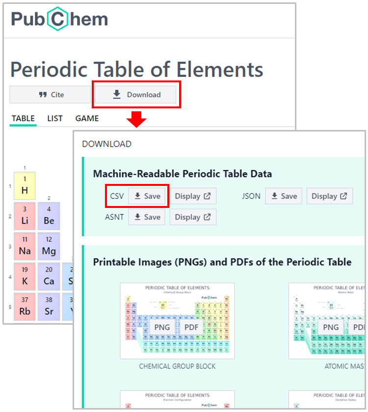
The data underlying the PubChem Periodic Table and Element Pages are freely available for download. This Jupyter notebook demonstrates how to download the properties of chemical elements and visualize the periodicity of those properties. The data used in this notebook can be downloaded from the PubChem Periodic Table (https://pubchem.ncbi.nlm.nih.gov/periodic-table/), by clicking the DOWNLOAD button and then the CSV button.

Alternatively, the data can also be downloaded using a python script, as demonstrated below. Here, we use a python data analysis library called pandas. Using pandas, we can directly load the data from the web into a data frame.

import requests
import pandas as pd

url = "https://pubchem.ncbi.nlm.nih.gov/rest/pug/periodictable/CSV"
df = pd.read_csv(url)

df

	AtomicNumber	Symbol	Name	AtomicMass	CPKHexColor	ElectronConfiguration	Electronegativity	AtomicRadius	IonizationEnergy	ElectronAffinity	OxidationStates	StandardState	MeltingPoint	BoilingPoint	Density	GroupBlock	YearDiscovered
0	1	H	Hydrogen	1.008000	FFFFFF	1s1	2.20	120.0	13.598	0.754	+1, -1	Gas	13.81	20.28	0.000090	Nonmetal	1766
1	2	He	Helium	4.002600	D9FFFF	1s2	NaN	140.0	24.587	NaN	0	Gas	0.95	4.22	0.000179	Noble gas	1868
2	3	Li	Lithium	7.000000	CC80FF	[He]2s1	0.98	182.0	5.392	0.618	+1	Solid	453.65	1615.00	0.534000	Alkali metal	1817
3	4	Be	Beryllium	9.012183	C2FF00	[He]2s2	1.57	153.0	9.323	NaN	+2	Solid	1560.00	2744.00	1.850000	Alkaline earth metal	1798
4	5	B	Boron	10.810000	FFB5B5	[He]2s2 2p1	2.04	192.0	8.298	0.277	+3	Solid	2348.00	4273.00	2.370000	Metalloid	1808
...	...	...	...	...	...	...	...	...	...	...	...	...	...	...	...	...	...
113	114	Fl	Flerovium	290.192000	NaN	[Rn]7s2 7p2 5f14 6d10 (predicted)	NaN	NaN	NaN	NaN	6, 4,2, 1, 0	Expected to be a Solid	NaN	NaN	NaN	Post-transition metal	1998
114	115	Mc	Moscovium	290.196000	NaN	[Rn]7s2 7p3 5f14 6d10 (predicted)	NaN	NaN	NaN	NaN	3, 1	Expected to be a Solid	NaN	NaN	NaN	Post-transition metal	2003
115	116	Lv	Livermorium	293.205000	NaN	[Rn]7s2 7p4 5f14 6d10 (predicted)	NaN	NaN	NaN	NaN	+4, +2, -2	Expected to be a Solid	NaN	NaN	NaN	Post-transition metal	2000
116	117	Ts	Tennessine	294.211000	NaN	[Rn]7s2 7p5 5f14 6d10 (predicted)	NaN	NaN	NaN	NaN	+5, +3, +1, -1	Expected to be a Solid	NaN	NaN	NaN	Halogen	2010
117	118	Og	Oganesson	295.216000	NaN	[Rn]7s2 7p6 5f14 6d10 (predicted)	NaN	NaN	NaN	NaN	+6, +4, +2, +1, 0, -1	Expected to be a Gas	NaN	NaN	NaN	Noble gas	2006

118 rows × 17 columns

df.shape      # Check the dimension of the data frame (the number of rows, the number of columns)

(118, 17)

df.columns    # Check the available information.

Index(['AtomicNumber', 'Symbol', 'Name', 'AtomicMass', 'CPKHexColor',
       'ElectronConfiguration', 'Electronegativity', 'AtomicRadius',
       'IonizationEnergy', 'ElectronAffinity', 'OxidationStates',
       'StandardState', 'MeltingPoint', 'BoilingPoint', 'Density',
       'GroupBlock', 'YearDiscovered'],
      dtype='object')

In some charts generated in this notebook, data will be color-coded using the information on the period of an element (i.e., the row on the periodic table where an element appears). However, as shown in the above code cell, this information is not available in the data frame. Therefore, we add it to the data frame.

Period = [None] * 118

for i in range(0,len(Period)):

    an =i + 1             # Atomic number

    if (1 <= an) & (an <= 2) :
        Period[i] = "Period 1"
    elif (3 <= an) & (an <= 10) :
        Period[i] = "Period 2"
    elif (11 <= an) & (an <= 18) :
        Period[i] = "Period 3"
    elif (19 <= an) & (an <= 36) :
        Period[i] = "Period 4"
    elif (37 <=an ) & (an <= 54) : 
        Period[i] = "Period 5"
    elif (55 <= an) & (an <= 86) :
        Period[i] = "Period 6"
    elif (87 <= an) & (an <= 118) :
        Period[i] = "Period 7"

df["Period"] = Period

Now let’s import matplotlib and seaborn for data visualization.

import matplotlib.pyplot as plt
import seaborn as sns

sns.set_style("darkgrid")

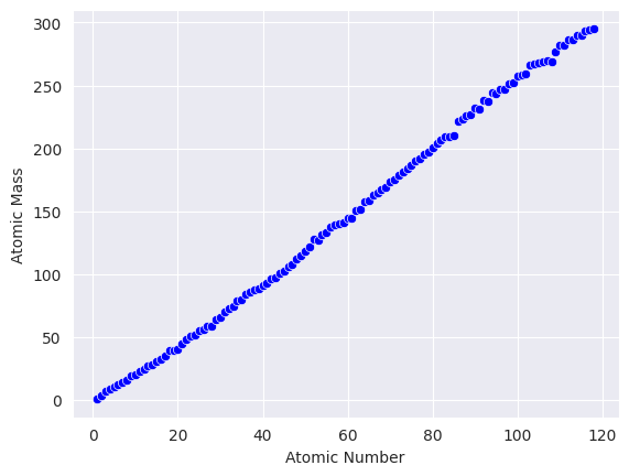
1. Atomic Mass

ax=sns.scatterplot(x=df.AtomicNumber, y=df.AtomicMass, color='Blue')
ax.set(xlabel='Atomic Number')
ax.set(ylabel='Atomic Mass')

[Text(0, 0.5, 'Atomic Mass')]

2. Ionization Energy, Electron Affinity & Electronegativity

Now we want to look into the periodicity of the ionization energy, electron affinity, and electronegativity among the chemical elements. These properties are not known for some elements, especially for elements heavier than Lr (Atomic Number=103), as identified in the following code cell.

df[(df.IonizationEnergy.isnull()) & (df.ElectronAffinity.isnull()) & (df.Electronegativity.isnull())][['AtomicNumber', 'Symbol','IonizationEnergy','ElectronAffinity','Electronegativity']]

	AtomicNumber	Symbol	IonizationEnergy	ElectronAffinity	Electronegativity
103	104	Rf	NaN	NaN	NaN
104	105	Db	NaN	NaN	NaN
105	106	Sg	NaN	NaN	NaN
106	107	Bh	NaN	NaN	NaN
107	108	Hs	NaN	NaN	NaN
108	109	Mt	NaN	NaN	NaN
109	110	Ds	NaN	NaN	NaN
110	111	Rg	NaN	NaN	NaN
111	112	Cn	NaN	NaN	NaN
112	113	Nh	NaN	NaN	NaN
113	114	Fl	NaN	NaN	NaN
114	115	Mc	NaN	NaN	NaN
115	116	Lv	NaN	NaN	NaN
116	117	Ts	NaN	NaN	NaN
117	118	Og	NaN	NaN	NaN

Therefore, let’s make a new data frame that does not have those elements without the Ionization energy, electron affinity, and electronegativity data.

df_tmp = df.dropna(axis=0, how='all', subset=['IonizationEnergy','ElectronAffinity','Electronegativity'])

df_tmp.shape

(103, 18)

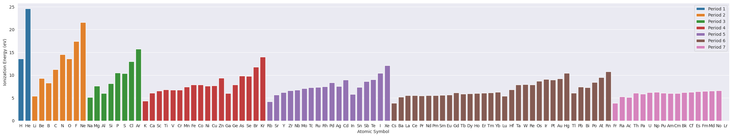
2.1. Ionization Potential

plt.figure(figsize=(30,5))
ax=sns.barplot(data=df_tmp, x="Symbol", y="IonizationEnergy", hue="Period", dodge=False)
ax.set(xlabel="Atomic Symbol", ylabel="Ionization Energy (eV)")
plt.legend(loc='upper right');

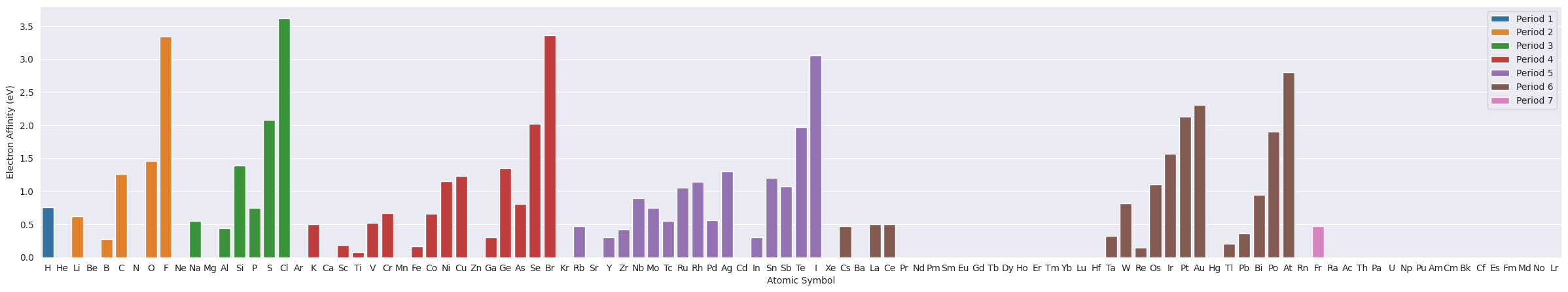
2.2. Electron Affinity

plt.figure(figsize=(30,5))
ax=sns.barplot(data=df_tmp, x="Symbol", y="ElectronAffinity", hue="Period", dodge=False)
ax.set(xlabel="Atomic Symbol", ylabel="Electron Affinity (eV)")
plt.legend(loc='upper right');

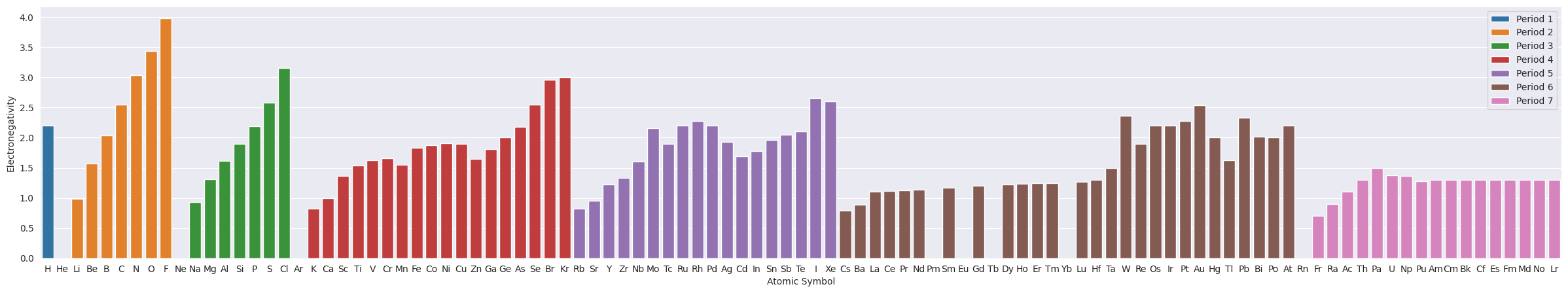
2.3. Electronegativity

plt.figure(figsize=(30,5))
ax=sns.barplot(data=df_tmp, x="Symbol", y="Electronegativity", hue="Period", dodge=False)
ax.set(xlabel="Atomic Symbol", ylabel="Electronegativity")
plt.legend(loc='upper right');

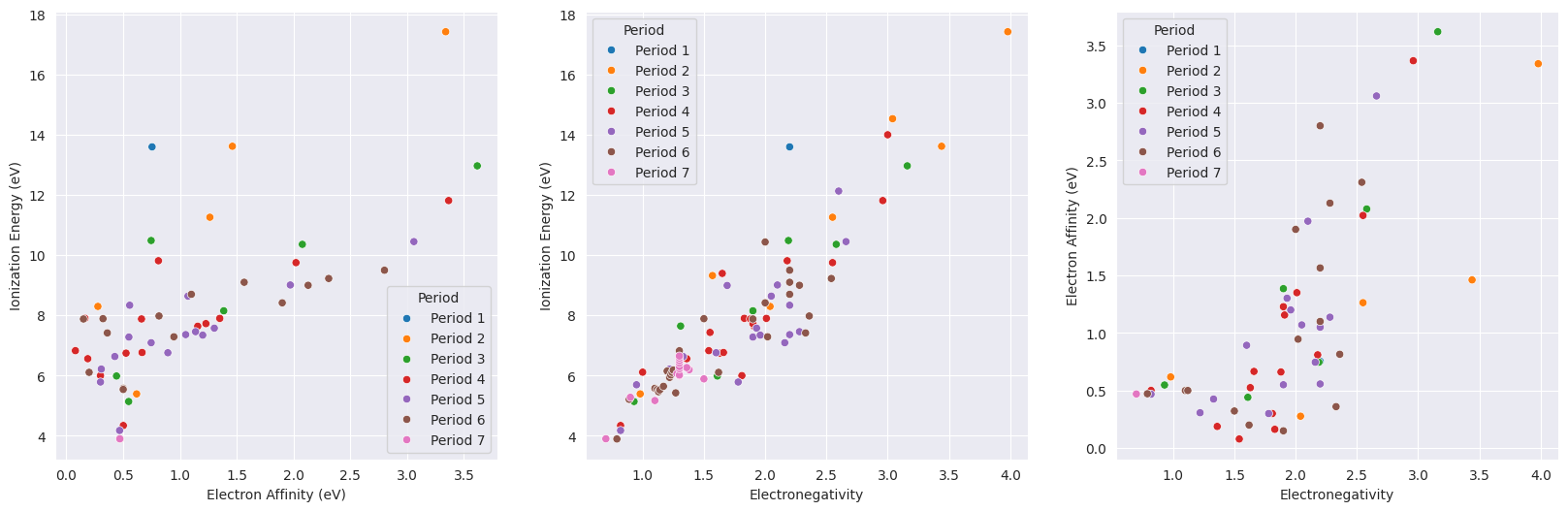
2.4. Comparison between Ionization Energy, Electron Affinity, and Electronegativity

fig, axs = plt.subplots(ncols=3,figsize=(20,6))

sns.scatterplot(data=df_tmp, x="ElectronAffinity", y="IonizationEnergy", hue="Period", ax=axs[0])
axs[0].set(xlabel="Electron Affinity (eV)", ylabel="Ionization Energy (eV)")

sns.scatterplot(data=df_tmp, x="Electronegativity", y="IonizationEnergy", hue="Period", ax=axs[1])
axs[1].set(xlabel="Electronegativity", ylabel="Ionization Energy (eV)")

sns.scatterplot(data=df_tmp, x="Electronegativity", y="ElectronAffinity", hue="Period", ax=axs[2])
axs[2].set(xlabel="Electronegativity", ylabel="Electron Affinity (eV)");

3. Melting Point and Boiling Point

Now let’s visualize the melting and boiling points of chemical elements. These data are not available for all compounds, so we want to exclude those elements without the necessary data.

df[(df.MeltingPoint.isnull()) & (df.BoilingPoint.isnull())][['AtomicNumber', 'Symbol','MeltingPoint','BoilingPoint']]

	AtomicNumber	Symbol	MeltingPoint	BoilingPoint
103	104	Rf	NaN	NaN
104	105	Db	NaN	NaN
105	106	Sg	NaN	NaN
106	107	Bh	NaN	NaN
107	108	Hs	NaN	NaN
108	109	Mt	NaN	NaN
109	110	Ds	NaN	NaN
110	111	Rg	NaN	NaN
111	112	Cn	NaN	NaN
112	113	Nh	NaN	NaN
113	114	Fl	NaN	NaN
114	115	Mc	NaN	NaN
115	116	Lv	NaN	NaN
116	117	Ts	NaN	NaN
117	118	Og	NaN	NaN

The elements with an atomic number greater than 103 do not have melting and boiling point data. Therefore, we want to exclude those elements by using the df_tmp data frame, which was used previously to create the charts for the ionization potential, electron affinity, and electronegativity.

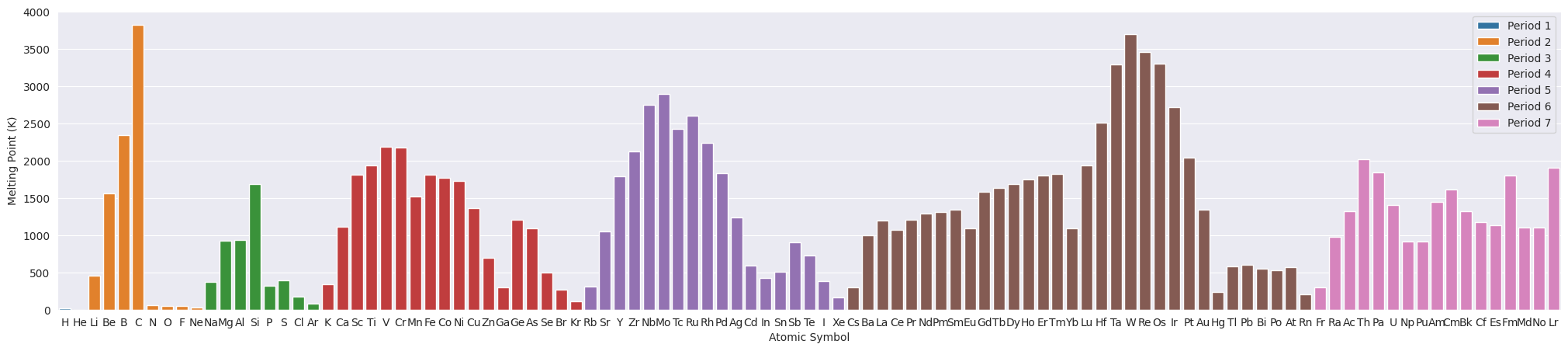
3.1. Melting Point

plt.figure(figsize=(25,5))
ax=sns.barplot(data=df_tmp, x="Symbol", y="MeltingPoint", hue="Period", dodge=False)
ax.set(xlabel="Atomic Symbol", ylabel="Melting Point (K)")
plt.legend(loc='upper right');

3.2. Boiling Point

plt.figure(figsize=(25,5))
sns.barplot(data=df_tmp, x="Symbol", y="BoilingPoint", hue="Period", dodge=False)
ax.set(xlabel="Atomic Symbol", ylabel="Boiling Point (K)")
plt.legend(loc='upper right');

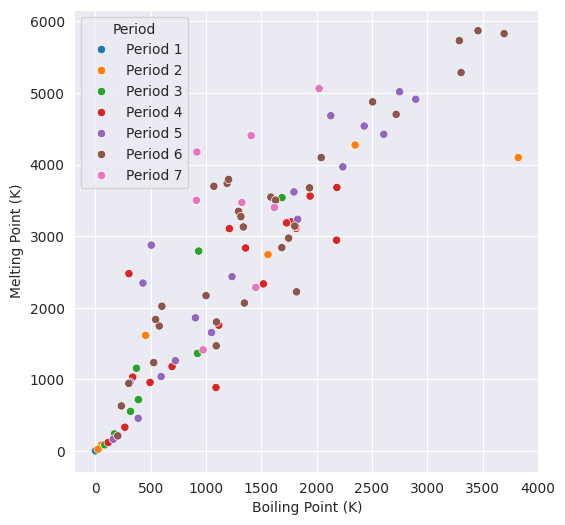
3.3. Comparison between Melting and Boiling Points

plt.figure(figsize=(6,6))
ax=sns.scatterplot(data=df, x="MeltingPoint", y="BoilingPoint", hue="Period")
ax.set(xlabel="Boiling Point (K)", ylabel="Melting Point (K)");

4. Density

Now let’s look into the density of chemical elements. The density data used here are measured at STP (standard temperature and pressure, 0 °C and 1 atm).

plt.figure(figsize=(25,5))
ax=sns.barplot(data=df_tmp, x="Symbol", y="Density", hue="Period", dodge=False)   # Use df_tmp to exclude the elements without relevant data.
ax.set(xlabel="Atomic Symbol", ylabel="Density ($g/cm^{3}$)");

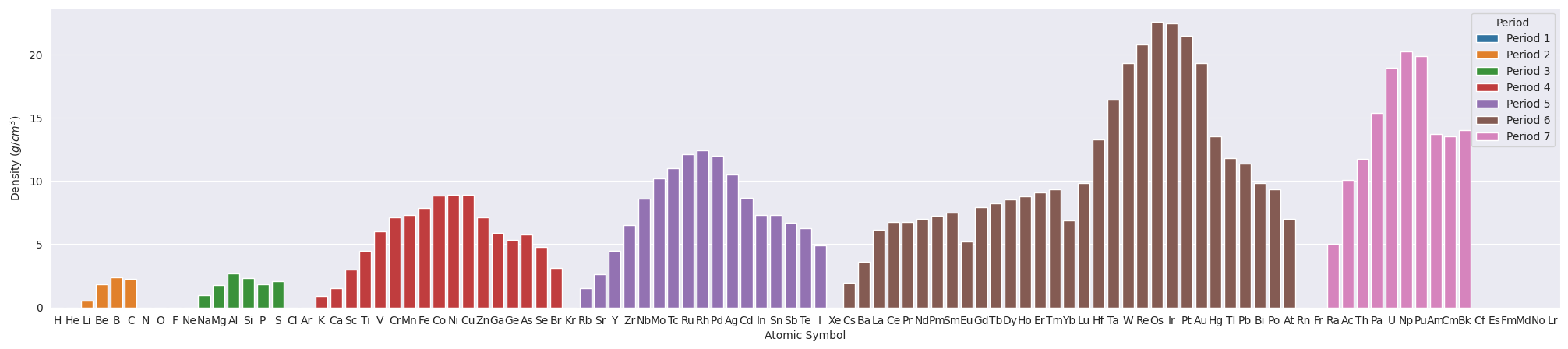
Some elements have very small density values, less than 0.5 g/cm³. This is also shown in the following histogram.

import numpy as np

bins=np.arange(0,25,0.5).tolist()    # list from 0 to 25 with an increment of 0.5
ax = sns.histplot(data=df_tmp, x='Density', bins=bins)
ax.set(xlabel="Density ($g/cm^{3}$)");

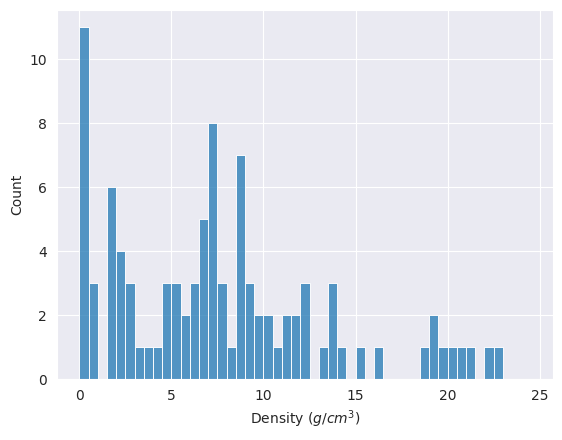
df_tmp[ df_tmp.Density < 0.5 ][['AtomicNumber','Symbol','Density','StandardState']]

	AtomicNumber	Symbol	Density	StandardState
0	1	H	0.000090	Gas
1	2	He	0.000179	Gas
6	7	N	0.001251	Gas
7	8	O	0.001429	Gas
8	9	F	0.001696	Gas
9	10	Ne	0.000900	Gas
16	17	Cl	0.003214	Gas
17	18	Ar	0.001784	Gas
35	36	Kr	0.003733	Gas
53	54	Xe	0.005887	Gas
85	86	Rn	0.009730	Gas

All these elements with densities < 0.5 g/cm³ exist as gas at STP.