Structured UV/Vis (meta)data for small molecule characterisation

Structured UV/Vis (meta)data for small molecule characterisation#

1. Objectives#

To provide guidance on the minimum set of metadata required for publishing UV/Vis spectroscopic data as supplementary information to support compound characterisation using the Beer-Lambert Law. To apply the FAIR principles for data management to produce digital data objects that contain raw, spectral and metadata to enable current and future researchers in the reanalysis and visualisation of UV/Vis spectroscopic data.

2. Target audience#

Researchers who routinely work with a user interface (spreadsheet) for preparation of supplementary material to support compound characterisation for publication: authors who aim to improve the FAIRness of their published supporting data.

FAIR data management refers to the IUPAC FAIRSpec standard: IUPAC specifications for the findability, accessibility, interoperability and reusability of spectroscopic data in chemistry.

3. Structuring the (meta)data#

3.1 File formats#

Textual metadata should (typically) be provided as a README.txt file.

Instrument–specific file formats should not be used for storage of the raw spectroscopic dataset. If JCAMP-DX is a fully supported format of the spectrophotometer, then the sample level metadata available in the raw data file could be user–defined or mandatory. The metadata content also depends on mapping from the spectrophotometer native software to JCAMP-DX. Sample level metadata should be supplemented using the file structure defined in 3.2 below.

The file formats recommended here are not exhaustive. For data reuse and preservation, all file formats must be non-proprietary, and associated software open source (maintained). Files should be uncompressed and unencrypted.

3.2 File hierarchy#

Raw Data
Content	Definition	Priority	Format
Data matrix (with or without column headings)	Spectrophotometer output as tabular data (absorbance and wavelength)	Essential	CSV (.csv) JCAMP–DX (.jdx)
Sample level metadata
Content	Definition	Priority	Format
Sample ID	Identifier for the sample which is unique within the project	Essential	Plain text (.txt) XML (.xml) R Markdown (.rmd) Jupyter Notebook Markdown (.ipynb)
Linking sample ID	Provenance identifier for the sample in the associated process capture document (digital or paper notebook)	Essential
Data labels (if absent from the data matrix)	Description and units for the tabular raw data columns	Essential
Sample concentration, solvent, optical path length, user ID and date/time of collection	Experimental parameters	Essential
Chemical structure	Chemical structure identifier in the form of an alphanumeric text string	Essential	InChI SMILES
Chemical structure	SMILES validation	Desirable	Toolkit(version) identifier
Analysis level metadata
Content	Definition	Priority	Format
Processed data matrix	Tabular data: absorbance, wavelength, and molar absorptivity (ε); with data labels and units	Essential	CSV (.csv)
Data reporting: 1. Plot of the UV/Vis spectrum 2. λ_max and ε (Section 4)	The two key outputs required for publication.	Essential	R Markdown (.rmd) Jupyter Notebook Markdown (.ipynb)
Project level metadata
Content	Definition	Priority	Format
Study ID	Identifier(s) for the scientific study; funder’s project ID(s)	Desirable	Plain text (.txt) XML (.xml) R Markdown (.rmd) Jupyter Notebook Markdown (.ipynb)
Instrument ID	Spectrophotometer vendor and version.	Desirable
Data storage location	Link to the data storage location	Essential	URL for an open access repository deposition
Spectrophotometer calibration	Link to structured calibration data	Essential	URL for an open access repository deposition

4. Data reporting using Jupyter Notebook (Python)#

Publication of UV/Vis spectroscopic data for small molecule characterisation typically requires a plot of the spectrum, and accompanying values for the wavelength of maximum absorbance (𝜆_max) and associated molar extinction coefficient (ε). An exemplar procedure for FAIR data reporting using Jupyter Notebook is described below, suitable for a novice user without existing experience in the Python language.

The UV/Vis reference data file ‘sample_data.jdx’ for salicylic acid in JCAMP-DX format is from the NIST Standard Reference Database available from the NIST Chemistry WebBook.

4.1 The tools#

What is Python?#

From the official python website, Python.org:

Python is an interpreted, object-oriented, high-level programming language with dynamic semantics. Its high-level built in data structures, combined with dynamic typing and dynamic binding, make it very attractive for Rapid Application Development, as well as for use as a scripting or glue language to connect existing components together. Python’s simple, easy to learn syntax emphasizes readability and therefore reduces the cost of program maintenance. Python supports modules and packages, which encourages program modularity and code reuse. The Python interpreter and the extensive standard library are available in source or binary form without charge for all major platforms, and can be freely distributed.

What is Jupyter/a Jupyter Notebook?#

Jupyter (formerly IPython Notebook) is an open-source project that lets you easily combine MarkDown text and executable Python source code on one canvas called a notebook. They are both human-readable documents containing the analysis description and the results (figures, tables, etc.) as well as executable documents which run the code to perform the data analysis.

What is Anaconda?#

Anaconda can be thought of as a one-stop shop for all things Python and data science. It’s almost an umbrella; by downloading Anaconda you also get Python, Jupyter notebooks and a whole host of other useful programmes. It is also a package manager and virtual environment manager.

Installing the tools#

The easiest way to install Python is through the package and virtual environment manager Anaconda. Anaconda is free and open source and the Individual Edition can be installed from https://www.anaconda.com/.

Once Anaconda is installed you can create a virtual environment, load Jupyter into the environment and run this notebook.

Running the notebook (on your computer)#

Make sure Anaconda is installed on your computer
Use the Anaconda navigator (or the command line) to create a virtual environment
Enter the virtual environment
Install Jupyter Notebooks, Matplotlib and Numpy (all can be done through Anaconda)
Follow this link, for instructions to install jcamp https://pypi.org/project/jcamp/
Launch Jupyter, navigate to the file you stored this notebook in and launch this notebook
You can edit code chunks by clicking on them and typing
You can run code chunks by clicking on them and pressing play (in the banner above) or by pressing shift+enter

4.2 Exemplar code for data reporting#

First the packages we need are imported into the Jupyter notebook

# noinspection PyProtectedMember
!pip install jcamp                        # command to instruct Binder/Colab to install the jcamp package
from jcamp import jcamp_read              # Importing the jcamp_read() method from the jcamp package
import matplotlib.pyplot as plt           # Importing a plotting package
import numpy as np                        # Import the numerical python package for mathematical operations
import requests

Requirement already satisfied: jcamp in /opt/hostedtoolcache/Python/3.11.8/x64/lib/python3.11/site-packages (1.2.2)
Requirement already satisfied: numpy in /opt/hostedtoolcache/Python/3.11.8/x64/lib/python3.11/site-packages (from jcamp) (1.26.2)
Requirement already satisfied: datetime in /opt/hostedtoolcache/Python/3.11.8/x64/lib/python3.11/site-packages (from jcamp) (5.4)
Requirement already satisfied: zope.interface in /opt/hostedtoolcache/Python/3.11.8/x64/lib/python3.11/site-packages (from datetime->jcamp) (6.1)
Requirement already satisfied: pytz in /opt/hostedtoolcache/Python/3.11.8/x64/lib/python3.11/site-packages (from datetime->jcamp) (2023.3.post1)

Requirement already satisfied: setuptools in /opt/hostedtoolcache/Python/3.11.8/x64/lib/python3.11/site-packages (from zope.interface->datetime->jcamp) (65.5.0)

Next, specify the file path that your file is saved at, and use the jcamp_read() method to import the data into your script

file = requests.get('https://raw.githubusercontent.com/IUPAC/WFChemCookbook/main/book/files/sample_data.jdx')
file = file.content.splitlines()                    # split raw text into lines
file = [line.decode("utf-8") for line in file]      # decode the lines into UTF-8
data_dictionary = jcamp_read(file)                  # Store the contents of the jdx file in a python dictionary  

The data is extracted into a dictionary of key:value pairs. We can quickly see what it contains by showing the contents on screen. It’s obvious that the data we need is saved as x and y, however the units are nm for x, but logged for y.

data_dictionary # Show the contents of the dictionary on screen

{'title': 'Salicylic Acid',
 'jcamp-dx': 4.24,
 'data type': 'UV/VIS SPECTRUM',
 'origin': 'INSTITUTE OF ENERGY PROBLEMS OF CHEMICAL PHYSICS, RAS',
 'owner': 'INEP CP RAS, NIST OSRD\nCollection (C) 2007 copyright by the U.S. Secretary of Commerce\non behalf of the United States of America. All rights reserved.',
 'cas registry no': '69-72-7',
 'molform': 'C7H6O3',
 'mp': 158,
 'bp': '211(20)',
 'source reference': 'RAS UV No. 237',
 '$nist squib': '1963ERN/MEN230-240',
 '$nist source': 'TSGMTE',
 'spectrometer/data system': 'Unicam SP 500',
 'xunits': 'Wavelength (nm)',
 'yunits': 'Logarithm epsilon',
 'xfactor': 1.0,
 'yfactor': 1.0,
 'firstx': 247.1048,
 'lastx': 340.0658,
 'firsty': 3.14445,
 'maxx': 340.066,
 'minx': 247.105,
 'maxy': 3.19782,
 'miny': 1.25709,
 'npoints': 1449,
 '$ref author': 'Ernst, Z.L.; Menashi, J.',
 '$ref title': 'The spectrophotometric determination of the dissociation constants of some substituted salicylic acids',
 '$ref journal': 'Trans. Faraday Soc.',
 '$ref volume': 59,
 '$ref page': '230-240',
 '$ref date': 1963,
 'xypoints': '(XY..XY)',
 'end': '',
 'x': array([247.1048, 247.1574, 247.1657, ..., 334.0779, 334.1783, 340.0658]),
 'y': array([3.14445 , 3.182843, 3.112433, ..., 1.693346, 1.67324 , 1.25709 ])}

We will now extract the x and y components from the dictionary. We can specify two variables (which are named with descriptive and informative names) that will hold the data associated with x and y

wavelength = data_dictionary['x'] # Variable named 'wavelength' holding x values as seen in dictionary above
log_epsilon = data_dictionary['y'] # Variable named 'log_epsilon' holding y values as seen in dictionary above

Now, plot the results on a graph

plt.plot(wavelength, log_epsilon)                      # Plot the two variables as a line graph
plt.xlabel('Wavelength (nm)')                          # Set the name of the x-label
plt.ylabel(r'Log $\epsilon$ ($L\ mol^{-1}\ cm^{-1}$)') # Set the name of the y-label
plt.title('UV spectrum of salicyclic acid')            # Set the title of the graph
plt.grid()                                             # Show grid lines
plt.savefig('uvvis_metadata_fig.png')                  # Saves the figure to your current directory.
                                                       # File path can be updated to suit
plt.show()                                             # Plot the graph to the screen

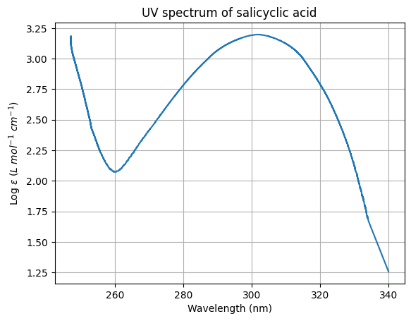
../_images/4f616e31310bb0f47387d9c899ef324593fd6003808614026e48b3e7a903e267.png

The plot has also been saved as an image.

In this example, for reporting of the molar extinction coefficient (ε) corresponding to λ_max we must first take the antilog

epsilon_array = 10**log_epsilon # Create an array and assign the antilog of log_epsilon 
                                # using numpys exp (exponential) method

arg_max = np.argmax(epsilon_array) # Use numpys arg max function to find the index of the largest y value
lambda_max = wavelength[arg_max] # Use this index to find the x value at max y
epsilon = epsilon_array[arg_max] # Find epsilon at this index 

print(f"{lambda_max:.1f} nm") # Printing output to screen to 1 d.p including proper units
print(f'{epsilon:.1f} L mol-1 cm-1') # Printing output to screen to 1 d.p including units 

301.6 nm
1577.0 L mol-1 cm-1

Now we create a function to apply the Beer Lambert law to convert Absorbance (A) to Absorptivity (ε) followed by a line of code to run the function.

# noinspection PyShadowingNames
def beer_lambert(absorbance, concentration, length):
    """
    Doc String
    ----------
    
    Calculates the molar absorptivity (epsilon) using the Beer-Lambert Law.
    
    The Beer-Lambert Law states that the absorbance (Absorbance) of a solution is directly proportional 
    to the concentration (concentration) of the absorbing species and the path length (length) of the 
    light through the solution. 
    
    Parameters:
    -----------
    
        absorbance (float): The measured absorbance of the solution
        concentration (float): The concentration of the absorbing species in the solution, in molar
        length (float): The path length of the light through the solution, in cm.
        
    Returns:
    --------
    
        epsilon (float): The molar absorptivity of the solution.
    
    """
    
    epsilon = absorbance/(concentration*length)
    
    return epsilon

absorbance = 1 # Edit to your own value
concentration = 2 # Edit to your own value
length = 3 # Edit to your own value

epsilon = beer_lambert(absorbance, concentration, length) # Replace each of the parameters, absorbance, 
                                                          # concentration and length with your own numbers.

print(f'The molar absorptivity (ε) is: {epsilon:.3f} L mol-1 cm-1')

The molar absorptivity (ε) is: 0.167 L mol-1 cm-1

5. Glossary of Python terms#

Package#

When developing a Python script, it’s often necessary to use functionality that is not included in the Python standard library. One way to access this additional functionality is by importing Python packages into your script. These packages, also known as modules, provide pre-built functionality and code that can be easily integrated into your script, saving you the time and effort of having to write everything from scratch. They can include functions, classes, or other objects that are ready to use or extend, and are written by other developers to solve specific problems or tasks. In addition, importing packages can also help to keep your code organized and maintainable, by breaking it up into reusable and functional blocks. In summary, we import packages into scripts to leverage pre-built functionality and take advantage of the expertise of the Python community, allowing us to focus on the specific problem we are trying to solve.

Comment#

In Python, a comment is a piece of text that is ignored by the interpreter when the code is executed. Comments are used to explain the purpose and logic of the code, and to make it easier for other people (or yourself) to understand and maintain the code. Comments can be a single line or span multiple lines and can start with a # symbol or be encapsulated by tiple quotes “”” “””. The text within the comment is only intended for human readers. Comments are very useful to add explanations and context to code, also it can help to keep track of the progress, problems or ideas you had when working in a script. Use them liberally.

Method#

A method is a function that is associated with an object. It is defined inside a class, and it can access and manipulate the attributes and state of the object it is associated with. Methods contain functionality that is often useful for the work you are doing, e.g. def for beer_lambert in the exemplar code above (section 4)

Data Structure#

In Python (and in computer science in general), a data structure is a way of organizing and storing data in a computer’s memory so that it can be efficiently accessed and modified.

Float#

A float (short for “floating-point number”) is a type of numeric data that can represent decimal values.

Function#

In Python, a function is a block of organized, reusable code that performs a specific task. Functions provide a way to organize your code into logical, modular chunks that can be easily reused and tested.

A Python function is defined using the def keyword, followed by the function name, a pair of parentheses (), and a colon :. The code inside the function is indented under the definition line.

Dictionary#

A dictionary is a built-in data structure that stores a collection of key-value pairs, where each key is unique. Dictionaries are also commonly known as associative arrays or hash maps. They are similar to lists or arrays in other programming languages, but the elements in a dictionary are accessed via keys rather than an index.

Variable#

In Python, a variable is a named location in memory that is used to store a value. A variable can be thought of as a “container” that holds a value, and the value can be of any data type (e.g., a number, a string, a list, etc.).

To create a variable in Python, you simply give it a name and assign a value to it using the assignment operator (=).

Doc String#

A docstring in Python is a string that appears at the top of a module, class, or function definition. Docstrings are used to provide a brief description of what the code does, as well as any information on the arguments, return values, and other details of the code.

Virtual Environment#

You may have multiple Python projects happening at once. A virtual environment is a named, isolated copy of Python that has its own files and packages. Anything done inside a virtual environment is specific to that environment and won’t affect any other projects. All the dependencies and packages you install will be sandboxed inside the environment you are using. You should therefore have a separate virtual environment for each separate project.